The $50k question for Bayes' Theorem [MODEL: part 2 of 3]

Here's a somewhat disturbing fact: in the city of San Francisco, if you are a single making under $60k/year you qualify for low-income housing. It's probably safe to assume that the average person working in San Francisco has a higher salary than someone in Baton Rouge, LA. While were at it, I think its also likely that individuals who are older and, hence, have worked more years will have a higher income. In fact, a census study done in 1994 asked these types of questions with the goal to determine if they could predict whether a given person earned more or less than $50k/year.

The data we will use for this study comes from the UCI machine learning repository, which houses a large set of data which is great for learning and testing different types of modeling techniques. The data we will be working with contains 14 data features which we will use to predict the likelihood a given individual has an income greater than $50k or less than (or equal to) $50k. You can find this census income data set here.   A description of the data is as follows:

• feature data is of type categorical or integer
• number of instances = 48842
• number of features = 14
• income class (dependent or response variable): >$50k or <=$50k

The details of the data at the feature-level is as follows:

• age: continuous value (years)
• workclass: private, federal-gov, local-gov, never-worked, etc.....
• fnlwgt: continuous demographic index value
• education: high-school, college, associates degree, PhD, etc
• education-num: (number of years educated)
• marital-status: single, married, divorces, etc
• occupation: Tech-support, Craft-repair, Other-service, Sales, etc
• relationship: Wife, Own-child, Husband, Not-in-family, etc
• race: White, Asian-Pac-Islander, Black, etc
• sex: Male, Female
• capital-gain: continuous value (dollars) 
• capital-loss: continuous value (dollars)
• hours-per-week: continuous value (hours)
• native-country: United-States, Cambodia, England, Puerto-Rico, Canada, etc

We will attempt to use Bayes' Theorem (Formal Explanation of Bayes' Theorem)

with the aforementioned 14 features to accurately predict an individuals income as >$50k or <=$50k.

As promised in the previous post, here is a quick and simple derivation of Bayes' Theorem since we will be actually applying it in this post (the MODEL portion of the series):

 = Probability of an event A & B occurring together


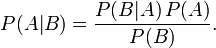
The conditional probability of event A occurring given B has occurred can also be thought of as the probability of both events A & B occurring together divided by the probability of event B occurring alone. The conditional probability of event B, given A has occurred can be similarly found. Formally:





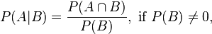
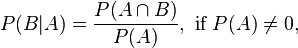
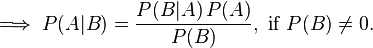
Now that we have expressed both P(A | B) and P(B | A) with the same numerator, we can simplify:



Then, dividing by P(B) yields the familiar form of Bayes' Theorem:



An important fact about using Bayes' theorem for classification (i.e. NB-classifiers) is that it requires the data to be discrete. In fact, the application of Bayes' Theorem used for this problem is often referred to as a multinomial naive bayes (MNB) classifier. THINK back to the first post of this series on Bayes' Theorem: all the probabilities (prior or conditional) were all computed assuming discrete values for the features. In the event you have a mixed set of features which are discrete and continuous, you can always discretize your continuous features (optimally discretizing features will be the topic of a future Think, Model, Code.... blog).

Okay, enough derivations. Let's return to the problem of predicting the income class of individuals. A good first step when looking at a new data set is look at the distribution of feature values. For this data set, of particular interest lies in the "age" feature. Age takes on many values (~ 80-100 values or years), while our response feature (income  >$50k or <=$50k) is binary. So let's plot a histogram and take a peek at the age distribution of individuals in this census:

Clearly there is a skew in the distribution towards younger individuals. The key here is to look at how age distributions change as a function of the two income classes (<=$50k  or >$50k).

Just as we suspected in the beginning of this post, there is a clear difference in age distribution. Younger individuals tend to make less money, as they have likely worked fewer years, whereas the peak age for the higher income earners is around the mid-40's and early-50's. Using this analysis, we can suggest a quantization of age from a nearly continuous feature to one that takes on fewer discrete values (NB-classifiers work best when you have the fewest values possible for discrete features while minimizing the information lost). Knowing that we would like to have discrete values representing the lower age groups and middle age groups, we can justifiably use ~ 6 discrete values corresponding to age "bins" which capture most the correlation with income class. If we have more than 6 feature values we start to lose correlation to the response feature (income) and likewise for fewer feature values. 6 features maximizes the correlation between age and income class. The new 6 values for age are such that anyone with an age between [17,29] would be given the age label = 1, age between [30,41] given age label = 2, age between [42-53] gets label = 3, and so on. Some of you may have noticed that basically the spacing is age bins of 11 years, this not by chance but the spacing that is "optimal." Instead of having ~90-100 different age possibilities, there are now just 6! Not only does this make computing the probabilities faster, but easier to interpret! (Unsurprisingly, this will also make computation time on in a computer program significantly faster).

Following this same type of rationale for studying the features with respect to the income class, we can determine different levels of discretization for any of the continuous features.

These continuous features were converted to discrete features with the corresponding new values:
age:                    [18-29], [30-41], [42-53], [54-65], [66-77], [77+]          --> 0,1,2,3,4,5
fnlwgt:               [13770-504081], [504082-994393], [994394,1484705] -- > 0,1,2
education-num:  [1,4], [5-7], [8-10], [11-13], [16+]                                  -- > 0,1,2,3,4
capital-gain:       [0-33333], [33334,66666], [66667,99999]                     --> 0,1,2
capital-loss:        [0-1089], [1090-2178], [2179-3267], [3268-4356]         --> 0,1,2,3
hours-per-week: [1-33.66], [33.67-66.33], [66.34-99]                              --> 0,1,2

We now have a fully discrete data set which can be used to train a NB-classifier (this amounts to finding the prior probabilities for the income classes and conditional probabilities). Training the NB-classifier is only part of the story. There's also a need to test the model against possibly overfitting the data and ensuring generalization of the classifier and accurate predictions. This process of training and testing a model is popularly known as cross-validation.

The UCI machine learning repository suggests we use 2/3 of the data for training and 1/3 of the data for testing. After removing rows in the data which have missing feature values, the final row count should go from 32561 --> 30162. Your training and test sets should be, approximately ~20000 training samples, and ~ 10000 test samples. Training essentially amounts to a scaled up version of what we did in the previous post: calculate prior and conditional probabilities for all 14 features against income class. The result of all the probabilities computed is what I refer to as a 3-dimensional "probability cube."

Here the "front" cube slice would be all the conditional probabilities (the probabilities are not the actual values) with respect to the income class (>$50k) while the "back" cube slice are the conditional probabilities with respect to (<=$50k). The table is used like this: A person in the first age "bin" has conditional probabilities of being in the income class (>$50k) of 6.5% and income class (<=$50k) of 12.5%. In other words, someone in the first age bin is twice as likely to be in the lower income class than the higher income class.

Let's look at the feature Native-Country. Someone from the 4th value of "native-country" has a 0.9% chance of being in the higher income class vs. 0.6% for the lower income class (this country happens to be Germany). Furthermore, just as we also did in the previous post, finding the conditional probability of being in either income class with respect to any number of features is simply a multiplicative computation. For example, someone with age = 1 and native-country=1, would have the resulting or posterior probabilities below:

P(>$50k) * P(Age_bin==1 | Income== >$50k) * P(Native-Country==1 | Income== >$50k) =

0.25 * 0.065 * 0.064 = 0.00104  (un-normalized)

P(<=$50k) * P(Age_bin==1 | Income== <=$50k) * P(Native-Country==1 | Income== <=$50k) =

0.75 * 0.125 * 0.105 = 0.00984 (un-normalized)

Consider what the results mean. For a person that is relatively young (Age = 1 is the lowest age "bin") and is from Native-Coutry = 1 (Puerto Rico), the odds lie nearly a 10-to-1 for them being in the lower income class vs. higher income class. 

Clearly, there are useful insights and interpretations from the Bayes' Model created. The take-home from all this: the meat of Naive-Bayes' (NB) Classifiers is the probability cube created looking at "past" events. Here, "training" data represents "past" events and the future (or individuals whose income class is taken as unknown) is represented by the "test" data. To make predictions on individuals which have unknown income class, we simply find or "look up" their corresponding conditional probabilities (as we did above) then determine which income class "wins" using the value of relative un-normalized probability. 

Coming up in part 3 [CODE portion] of this series:

1. Creating a python script to execute a NB-classifier on the above train and test data sets!